Exercises
For issues, bugs, proposals or remarks, visit the issue tracker.
Tutorial Data Set
You can find the data (data_qgis.zip) on the bitbucket download page.
We will use five areas in Heverlee Forest, situated near Leuven, BE.
For each forest patch (with numbers 15, 38, 64, 84 and 103) you will find:
- a false colour composite polyg_x.tif with 20 cm resolution
- an image polyg_x_100cm.tif with the infrared band at 100 cm resolution
- a vector file polyg_x.shp with the edges of the forest patch
Where x indicates the forest patch number.
Goal
We want to test if the Tree Density Calculator is a reliable estimator of tree densities.
It is important to have sufficient reference material (ground truth) to compare the results of the algorithm with. This reference material can be acquired for example in the field. In this exercise, we will use a remote sensing false colour composite image of 20 cm spatial resolution, to naively locate tree tops by hand.
In general, you will go through these steps for each forest patch:
- Acquire a reference data set and count the number of trees in the data set.
- Apply the Tree Density Calculator on a 100 cm and 200 cm resolution image, using two different sliding windows and again count the number of trees in the data set.
- Determine the relation between the reference data set and the Tree Density Calculator data set.
If there is a strong relationship between the two, we can prove that the Tree Density Calculator can be used as a measure of determining tree densities.
Step 1. Reference data set
Manually digitize the tree tops in QGIS. For this we need to create a new, empty vector file.
Load the image patch in QGIS (drag and drop or Add Raster Layer…).
Note: Coordinate reference system information should be EPSG:31370 - Belge 1972 / Belgian Lambert 72.
Load the forest patch boundaries (drag and drop or Add Vector Layer…). Again the CRS should be EPSG:31370.
Change the symbology: make sure there is no fill color and the boundaries are clearly visible.
Click Create Layer > New Shapefile Layer in the Layer menu. Give the file a name (e.g. polyg_x_reference), make sure it is a point layer and has EPSG:31370 as CRS. We won’t be saving attribute data so you don’t have to add any fields.
To start digitizing, select the new point layer in the table of contents and click Toggle editing in the Layers menu. Then click Add Feature: Capture Point in the Edit menu.
Now you can click on all the tree tops you see. QGIS will ask you for an ID. You can ignore this en simply click OK or press Enter. To delete a point, you can either undo an edit or use the Select Object tool and press Delete.
Don’t forget to save your edits on regular basis! You find the save button in the Layers menu.
Counting the number of trees is easy now. Just open the attribute table and count the number of items. Alternatively, right click on the layer in the table of contents and select Show number of objects.
Step 2. Forest patch area
To get the area of the forest patch. Use the Identify tool in QGIS. Click on the shapefile with the boundaries. A window with identification results should open. One of the derived statistics is the area, based on the cartesian coordinates.
Step 3. Test the Tree Density Calculator
Before we can do this, we still need a 200 cm resolution image. We will create it by degrading each 100 cm resolution image with a factor of 2.
In QGIS, do the following:
- Load the 100 cm resolution image.
- Use the Raster Alignment tool in the Raster menu. Use average as resampling method, leave the CRS at it’s invalid state (otherwise you get an error) and double the cell size (don’t just add ‘1’).
Now that you have both the 100 cm and 200 cm resolution images, you can use them in the Tree Density Calculator:
- Open either the 100 cm or 200 cm resolution image.
- Choose a window size. First try 5 pixels, next try 3 pixels. What is that in meters?
- Open the corresponding vector layer representing the area of interest.
As a result, we will have a point vector layer representing the tree canopies detected with the given window size and a copy of the input polygon vector layer with the following attributes:
- “Area_ha” the polygon area in ha,
- “TreeCount” the number of trees and
- “TreeDens” the tree density as number of trees per ha.
Step 4. Determine the relation between the reference data set and the Tree Density Calculator data set
Now you have for each forest patch the tree density counted by hand, and the tree density counted by the QGIS plugin. Use a program like Excel to create a scatterplot per window size and add a trend line. Display the trend’s equation and R2.
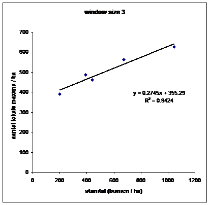
An example of a scatterplot of the tree densities (reference numbers on the x-axis and measurements on the y-axis)